
A quick post on how to build a control flow graph.
What is a CFG?
According to Wikipedia a CFG is “a representation, using graph notation, of all paths that might be traversed through a program during its execution“.
CFGs enable to represent functions in a convenient way and are used for instance by disassemblers (to better visualize the different possible execution paths) but also by compilers (dead code elimination) and other kind of tools. They are omnipresent when dealing with binaries.
The constituents of CFGs are called basic blocks (BB). A BB is a group of instructions that execute sequentially or “together” (when not considering exceptions that might occur). Control always enters a basic block at its first operation and exits at its last operation. Typically, the latter is a control transfer instruction, more specifically a JUMP or CJUMP.
One might ask: “If I encounter an instruction of the form: jmp rax
[A CFG] is ignoring the data values in registers and memory, and ignoring the arithmetic calculations.
In our case, as the content of eax depends on previous computations, we simply don’t consider this instructions in the construction of our CFG. We ignore it as we ignore any non CFLOW instructions. Therefore, we can conclude that JUMPs and CJUMPs that use indirect addressing will not be elligible to end BBs.
The implementation
Surreptitious Software authors gave a simple algorithm to build a CFG:
- Mark every instruction that can start a basic block as a leader:
- The first instruction is a leader;
- Any target of a branch is a leader;
- The instruction following a conditional branch (the fallthrough) is a leader.
- A basic block consists of the instructions from a leader up to, but not including, the next leader.
- Add an edge A → B if A ends with a branch to B or can fall through to B.
In order to get the meaning of each instruction, we must use a good disassembler: I’ve chosen Zydis for that matter.
I’ve decided to represent the basic blocks and the CFG like this:
typedef struct basic_block
{
    U64 leader;
    U64 tail;
    U64 targets[MAX_TARGETS];
    char* str;
} BB;

typedef struct control_flow_graph
{
    U64 bb_count;
    U64 leaders_table[MAX_BB];
    U64 bb_table[MAX_BB][1];
} CFG;
The str variable in the BB structure is dynamically allocated and is used to store the string representation of the basic block.leaders_table contains the addresses of each leaders and bb_table contains the addresses of each BB object: it’s a kind of key-value data structure where each BB can be retrieved in this way:
BB* get_bb_from_address(CFG* cfg, U64 address)
{
    return (BB*)*cfg->bb_table[address % MAX_BB];
}
This enables quick lookups (we do not have to iterate on a list) but some collisions may occur.
As it is more a POC that a robust and efficient implementation, I allowed myself to go through the whole disassembly twice. I’ve used the DOT language to represent the graph. One can use Graphviz’ dot program to generate an image from it (I’ve included a script, draw.sh, that do just that and displays the generated PNG).
Few examples
Example 1
A dummy assembly program:
007FFFFFFF400000 jnz 0x007FFFFFFF400002
007FFFFFFF400002 push rbp
007FFFFFFF400003 mov rbp, rsp
007FFFFFFF400006 sub rsp, 0x20
007FFFFFFF40000A mov qword ptr [rbp-0x18], 0x00
007FFFFFFF400012 mov qword ptr [rbp-0x20], 0x01
007FFFFFFF40001A cmp [rbp-0x18], rcx
007FFFFFFF40001E jnl 0x007FFFFFFF400056
007FFFFFFF400020 mov rax, [rbp-0x18]
007FFFFFFF400024 mov rax, [rsi+rax*1]
007FFFFFFF400028 cmp rax, 0x01
007FFFFFFF40002C jnz 0x007FFFFFFF400038
007FFFFFFF40002E mov qword ptr [rbp-0x08], 0xCA1C
007FFFFFFF400036 jmp 0x007FFFFFFF400040
007FFFFFFF400038 mov rax, [rbp-0x20]
007FFFFFFF40003C mov [rbp-0x08], rax
007FFFFFFF400040 mov qword ptr [rbp-0x20], 0xCA1C2
007FFFFFFF400048 mov rax, [rbp-0x08]
007FFFFFFF40004C mov [rbp-0x10], rax
007FFFFFFF400050 inc [rbp-0x18]
007FFFFFFF400054 jmp 0x007FFFFFFF40001A
007FFFFFFF400056 ret
007FFFFFFF400057 jnz 0x007FFFFFFF400053
Our program console output:
bkwg@sangria:~/bb$ ./compile_and_run.sh
>> Number of leaders: 9
 _____________ BB ____________
| LEADER: 0x07FFFFFFF400000   |
| END: 0x07FFFFFFF400003      |
|    |_ T0: 0x07FFFFFFF400005 |
|    |_ T1: 0x07FFFFFFF400005 |
 _____________________________

 _____________ BB ____________
| LEADER: 0x07FFFFFFF400005   |
| END: 0x07FFFFFFF400015      |
|    |_ T0: 0x07FFFFFFF40001D |
 _____________________________

 _____________ BB ____________
| LEADER: 0x07FFFFFFF400059   |
| END: 0x07FFFFFFF40005A      |
|    |_ T0: 0x07FFFFFFF400056 |
 _____________________________

 _____________ BB ____________
| LEADER: 0x07FFFFFFF400023   |
| END: 0x07FFFFFFF40002F      |
|    |_ T0: 0x07FFFFFFF400031 |
|    |_ T1: 0x07FFFFFFF40003B |
 _____________________________

 _____________ BB ____________
| LEADER: 0x07FFFFFFF40003B   |
| END: 0x07FFFFFFF40003F      |
|    |_ T0: 0x07FFFFFFF400043 |
 _____________________________

 _____________ BB ____________
| LEADER: 0x07FFFFFFF400031   |
| END: 0x07FFFFFFF400039      |
|    |_ T0: 0x07FFFFFFF400043 |
 _____________________________

 _____________ BB ____________
| LEADER: 0x07FFFFFFF400043   |
| END: 0x07FFFFFFF400057      |
|    |_ T0: 0x07FFFFFFF40001D |
 _____________________________

 _____________ BB ____________
| LEADER: 0x07FFFFFFF40001D   |
| END: 0x07FFFFFFF400021      |
|    |_ T0: 0x07FFFFFFF400023 |
|    |_ T1: 0x07FFFFFFF400059 |
 _____________________________

 _____________ BB ____________
| LEADER: 0x07FFFFFFF400056   |
| END: 0x000000000000000      |
 _____________________________


[+] Dumping to dot
[+] Done dumping dot to file: graph.dot
And finally the dot output:
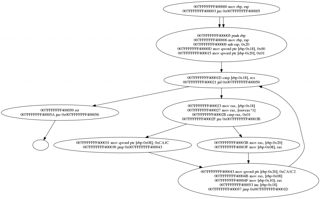
Ain’t it beautiful ?
Few questions that you may ask:
- – Why two edges from the first node?
- The BB ends with a conditional jump thus two execution paths are possible. But the target of the jump is equal to the fallthrough so both are aiming at the same node.
- – Ok, but then, why displaying both?
- – What is this empty node?
- The target of the branch is
0x07FFFFFFF400056which is not a ‘valid’ address (instruction overlapping) so the program simply represented an edge but didn’t display the disassembly from that address because I didn’t find it necessary.
- The target of the branch is
Example 2 – Comparison with ODA’s output
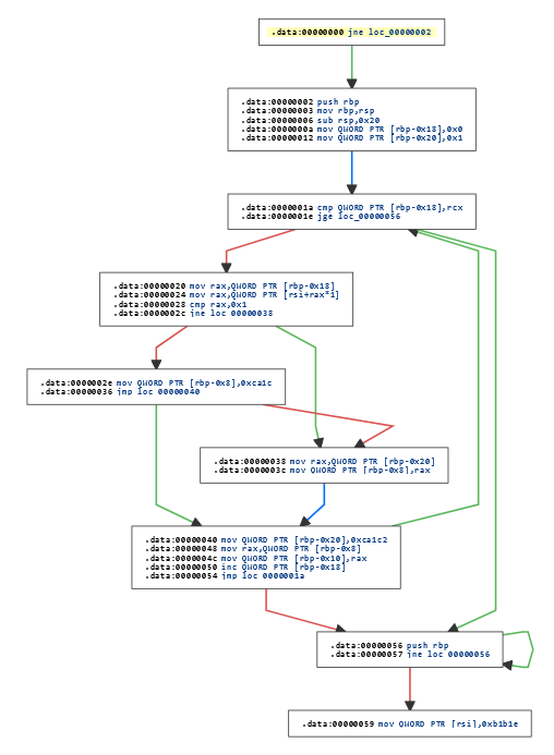
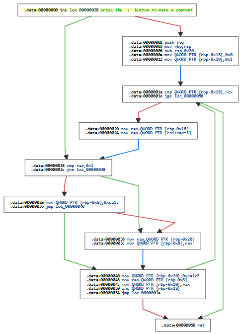
Here is another example, but now let’s compare our graph with ODA‘s:
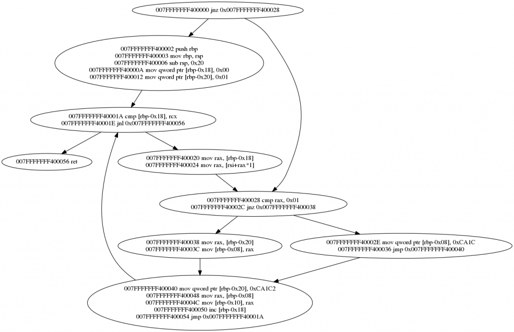
And ours:
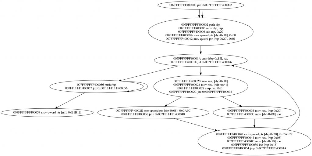
We can see that both graphs looks very similar… BUT an important difference is visible still. Indeed, ODA is displaying a branch where it shouldn’t: if we look at BBs that finish with a jmp, we can see that an edge representing a fallthrough is systematically displayed. As this is an unconditionnal control transfer instruction only one path is possible thus that extra edge shouldn’t appear.
Our graph doesn’t display these edges.
Example 3 – Comparison with ODA’s output 2
And a final example:
Conclusion
As I said previously, this program is more a POC than a robust/optimized tool, but I find the result satisfying enough. I may improve it in the future, in order to incorporate it in bigger projects.
The source code is available on my Github.